// [[Rcpp::depends(dqrng,BH,sitmo)]]
#include <Rcpp.h>
#include <dqrng_distribution.h>

auto rng = dqrng::generator<>(42);

// [[Rcpp::export]]
Rcpp::IntegerVector sample_prob(int size, Rcpp::NumericVector prob) {
  Rcpp::IntegerVector result(Rcpp::no_init(size));
  double max_prob = Rcpp::max(prob);
  uint32_t n(prob.length());
  std::generate(result.begin(), result.end(),
                [n, prob, max_prob] () {
                  while (true) {
                    int index = (*rng)(n);
                    if (dqrng::uniform01((*rng)()) < prob[index] / max_prob)
                      return index + 1;
                  }
                });
  return result;
} I have blogged about weighted sampling before. There I found that the stochastic acceptance method suggested by Lipowski and Lipowska (2012) (also at https://arxiv.org/abs/1109.3627) is very promising:
For relatively even weight distributions, as created by runif(n) or sample(n), performance is good, especially for larger populations:
sample_R <- function (size, prob) {
  sample.int(length(prob), size, replace = TRUE, prob)
}

size <- 1e4
prob10 <- sample(10)
prob100 <- sample(100)
prob1000 <- sample(1000)
bm <- bench::mark(
  sample_R(size, prob10),
  sample_prob(size, prob10),
  sample_R(size, prob100),
  sample_prob(size, prob100),
  sample_R(size, prob1000),
  sample_prob(size, prob1000),
  check = FALSE
)
knitr::kable(bm[, 1:6])| expression | min | median | itr/sec | mem_alloc | gc/sec |
|---|---|---|---|---|---|
| sample_R(size, prob10) | 229µs | 256µs | 3692.370 | 41.6KB | 2.016587 |
| sample_prob(size, prob10) | 316µs | 333µs | 2799.726 | 41.6KB | 2.017094 |
| sample_R(size, prob100) | 428µs | 446µs | 2112.141 | 52.9KB | 2.015402 |
| sample_prob(size, prob100) | 353µs | 367µs | 2534.683 | 47.6KB | 2.014851 |
| sample_R(size, prob1000) | 486µs | 513µs | 1858.395 | 53.4KB | 2.015613 |
| sample_prob(size, prob1000) | 360µs | 374µs | 2520.599 | 49.5KB | 2.016479 |
The nice performance breaks down when an uneven weight distribution is used. Here the largest element n is replaced by n * n, severely deteriorating the performance of the stochastic acceptance method:
size <- 1e4
prob10 <- sample(10)
prob10[which.max(prob10)] <- 10 * 10
prob100 <- sample(100)
prob100[which.max(prob100)] <- 100 * 100
prob1000 <- sample(1000)
prob1000[which.max(prob1000)] <- 1000 * 1000
bm <- bench::mark(
  sample_R(size, prob10),
  sample_prob(size, prob10),
  sample_R(size, prob100),
  sample_prob(size, prob100),
  sample_R(size, prob1000),
  sample_prob(size, prob1000),
  check = FALSE
)
knitr::kable(bm[, 1:6])| expression | min | median | itr/sec | mem_alloc | gc/sec |
|---|---|---|---|---|---|
| sample_R(size, prob10) | 161.75µs | 169.13µs | 5501.152611 | 41.6KB | 4.073419 |
| sample_prob(size, prob10) | 854.02µs | 906.83µs | 1060.873684 | 41.6KB | 0.000000 |
| sample_R(size, prob100) | 238.76µs | 252.51µs | 3637.956539 | 42.9KB | 4.073860 |
| sample_prob(size, prob100) | 7.08ms | 7.61ms | 130.633690 | 41.6KB | 0.000000 |
| sample_R(size, prob1000) | 469.83µs | 484.27µs | 1919.669187 | 53.4KB | 2.016459 |
| sample_prob(size, prob1000) | 71.98ms | 123.2ms | 9.646388 | 41.6KB | 0.000000 |
A good way to think about this was described by Keith Schwarz (2011).1 The stochastic acceptance method can be compared to randomly throwing a dart at a bar chart of the weight distribution. If the weight distribution is very uneven, there is a lot of empty space on the chart, i.e. one has to try very often to not hit the empty space. To quantify this, one can use max_weight / average_weight, which is a measure for how many tries one needs before a throw is successful:
- This is 1 for un-weighted distribution.
- This is (around) 2 for a random or a linear weight distribution.
- This would be the number of elements in the extreme case where all weight is on one element.
The above page also discusses an alternative: The alias method originally suggested by Walker (1974, 1977) in the efficient formulation of Vose (1991), which is also used by R in certain cases. The general idea is to redistribute the weight from high weight items to an alias table associated with low weight items. Let’s implement it in C++:
#include <queue>
// [[Rcpp::depends(dqrng,BH,sitmo)]]
#include <Rcpp.h>
#include <dqrng_distribution.h>

auto rng = dqrng::generator<>(42);

// [[Rcpp::export]]
Rcpp::IntegerVector sample_alias(int size, Rcpp::NumericVector prob) {
  uint32_t n(prob.size());
  std::vector<int> alias(n);
  Rcpp::NumericVector p = prob * n / Rcpp::sum(prob);
  std::queue<int> high;
  std::queue<int> low;
  for(int i = 0; i < n; ++i) {
    if (p[i] < 1.0)
      low.push(i);
    else
      high.push(i);
  }
  while(!low.empty() && !high.empty()) {
    int l = low.front();
    low.pop();
    int h = high.front();
    alias[l] = h;
    p[h] = (p[h] + p[l]) - 1.0;
    if (p[h] < 1.0) {
      low.push(h);
      high.pop();
    }
  }
  while (!low.empty()) {
    p[low.front()] = 1.0;
    low.pop();
  }
  while (!high.empty()) {
    p[high.front()] = 1.0;
    high.pop();
  }
  Rcpp::IntegerVector result(Rcpp::no_init(size));
  std::generate(result.begin(), result.end(),
                [n, p, alias] () {
                    int index = (*rng)(n);
                    if (dqrng::uniform01((*rng)()) < p[index])
                      return index + 1;
                    else
                      return alias[index] + 1;
                });
  return result;
}
First we need to make sure that all algorithms select the different possibilities with the same probabilities, which seems to be the case:
size <- 1e6
n <- 10
prob <- sample(n)
data.frame(
  sample_R = sample_R(size, prob),
  sample_prob = sample_prob(size, prob),
  sample_alias = sample_alias(size, prob)
) |> pivot_longer(cols = starts_with("sample")) |>
ggplot(aes(x = value, fill = name)) + geom_bar(position = "dodge2")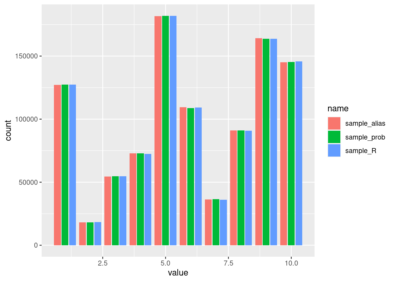
Next we benchmark the three methods for a range of different population sizes n and returned samples size. First for a linear weight distribution:
bp1 <- bench::press(
  n = 10^(1:4),
  size = 10^(0:5),
  {
    prob <- sample(n)
    bench::mark(
                  sample_R = sample_R(size, prob),
                  sample_prob = sample_prob(size, prob = prob),
                  sample_alias = sample_alias(size, prob = prob),
                  check = FALSE,
                  time_unit = "s"
    )
  }
) |>
  mutate(label = as.factor(attr(expression, "description")))
ggplot(bp1, aes(x = n, y = median, color = label)) +
  geom_line() + scale_x_log10() + scale_y_log10() + facet_wrap(vars(size))
For n > size stochastic sampling seems to work still very well. But when many samples are created, the work done to even out the weights does pay off. This seems to give a good way to decide which method to use. And how about an uneven weight distribution?
bp2 <- bench::press(
  n = 10^(1:4),
  size = 10^(0:5),
  {
    prob <- sample(n)
    prob[which.max(prob)] <- n * n
    bench::mark(
                  sample_R = sample_R(size, prob),
                  sample_prob = sample_prob(size, prob = prob),
                  sample_alias = sample_alias(size, prob = prob),
                  check = FALSE,
                  time_unit = "s"
    )
  }
) |>
  mutate(label = as.factor(attr(expression, "description")))
ggplot(bp2, aes(x = n, y = median, color = label)) +
  geom_line() + scale_x_log10() + scale_y_log10() + facet_wrap(vars(size))
Here the alias method is the fastest as long as there are more than one element generated. But when is the weight distribution so uneven, that one should use the alias method (almost) everywhere? Further investigations are needed …
References
Keith Schwarz. 2011. “Darts, Dice, and Coins.” https://www.keithschwarz.com/darts-dice-coins/.
Lipowski, Adam, and Dorota Lipowska. 2012. “Roulette-Wheel Selection via Stochastic Acceptance.” Physica A: Statistical Mechanics and Its Applications 391 (6): 2193–96. https://doi.org/10.1016/j.physa.2011.12.004.
Vose, M. D. 1991. “A Linear Algorithm for Generating Random Numbers with a Given Distribution.” IEEE Transactions on Software Engineering 17 (9): 972–75. https://doi.org/10.1109/32.92917.
Walker, Alastair J. 1974. “New Fast Method for Generating Discrete Random Numbers with Arbitrary Frequency Distributions.” Electronics Letters 10 (8): 127. https://doi.org/10.1049/el:19740097.
———. 1977. “An Efficient Method for Generating Discrete Random Variables with General Distributions.” ACM Transactions on Mathematical Software 3 (3): 253–56. https://doi.org/10.1145/355744.355749.